Computational modelling of the companion star and its interaction with Sol

psychegram said:

Well this is just stunning. Absolutely amazing work.

It seems that the simulations suggest a much smaller influx of cometary bodies than has in fact been observed. However, it seems (unless I am misinterpreting something) that the smallest perihelion you test is 100 AU. But according to the 98/07/04 transcript, perihelion is rather less than this:

A: They are moving in tandem with one another along a flat, elliptical orbital plane. Outer reaches of solar system are breached by passage of brown companion, thus explaining anomalies recently discovered regarding outer planets and their moons.
Q: (A) […] Elliptical orbit means there is perihelion and aphelion. I want to know what will be, or what was, or what is the closest distance between this brown star and the sun? What is perihelion? Can we know this, even approximately. Is it about one light year, or less or more?
A: Less, much less. Distance of closest passage roughly corresponds to the distance of the orbit of Pluto from Sun.
Q: (A) Okay. Now, this closest pass, is this something that is going to happen?
A: Yes.
Q: (A) And it is going to happen within the next 6 to 18 years?
A: 0 to 14.

Click to expand...

Now, ignoring the large perihelion increase in the number of Earth-crossing objects, which as you note is likely an artifact of the model originating in the use of a constant number density, it seems that the increase with perihelion distance (beyond about 300 AU) is quite strong. Therefore, how do the results change if perihelion is closer to 50 AU? And how do they change if the number density is more realistic?

Click to expand...

Thank you for your input psychegram, you are correct I was interested in what happens over long heliocentric distances. But it is obvious that until approx 200-300 AU the influx is almost constant therefore it would be interesting to see what happens for the closer approach. I will post the results shortly.

I will try to also increase the initial density but the exact value is largely unknown so for now I can only guess.

Inner works

Up until now a larger scale was observed up to 900 AU distance. Nonetheless the most important region is a region close to the outer planets coinciding with the Edgeworth-Kuiper belt because the region is very densely seeded by asteroids and planetesimals. It is speculated that the approximate number of comet sized bodies (2 km diameter) within 50 AU is 1010 [1].

To estimate the influx of bodies into inner solar system from the close encounters in the EK belt the bodies were seeded from 50 to 150 AU. The planar density of the bodies was chosen to be 2500 AU-2 because of two reasons. First the relationship on the spatial density is linear and it was shown that for the density the results are enough accurate. The second reason is the computing power which is sufficient for calculation of 100k bodies in acceptable time. The distance range was divided into smaller parts each with width 10 AU. Simulation for each one was performed so that each part contribution is identifiable. Nonetheless putting all these parts together a continuous domain is obtained and also the results would correspond to a continuous asteroid cloud. The companion was modeled with orbit in the plane of ecliptic and with perihelion distance roughly 40 AU.

References:
[1] Duncan, M. et al. The dynamical structure of the Kuiper belt. 1995, AJ, Vol. 110, No. 6.

The results are presented in Fig. 9 and Fig. 10 in similar fashion as in Fig. 6 and Fig. 7. The blue lines correspond to individual parts to which the whole interval was divided. There are 10 such lines with clearly identifiable peaks. The red line is a sum of all the contributions from the individual parts which together give continuous cloud.

On the x-axis is the estimated time of the companion arrival. It can be seen from both of the graphs that there is good agreement with the larger scale simulation for the distance 100 AU. Nonetheless the increase in the influx and density is even more dramatic when the 100 AU barrier is crossed.

For the 60/70 AU patch the destabilized tail was also included and is observable on the figure. This is because it kicked in early and it was natural to capture it. For the more distant patches these tails arrive long after the companion passed the perihelion, nonetheless they are present.

For the 50/60 AU patch an interesting phenomenon occurred because after the companion passed approximately 54 AU mark all of the asteroids that interacted with it were thrown off of the inner solar system. This is because the velocity vector of the companion at that distance is close to tangential direction in respect to the sun and the momentum of the asteroids given to them by the companion ejected them on an elliptical orbit with perihelion distance larger than 1 AU. For this patch there was no destabilized tail.
Nonetheless even when the asteroids with the initial heliocentric distance less than 54 AU do not interact with the inner solar system, the influx is still continuous because there is enough bodies that are still on approach, e.g. the destabilized tail.

I include below a figure of estimated time for the companion to reach the perihelion vs. its heliocentric distance for better understanding (Fig. 11).

For example it takes approximately 50 years for the asteroids with the heliocentric distance 100 AU to arrive to Earth after they were ejected by the companion from their stable orbits. And it takes approximately 28 years for the ones that are located at 60 AU from the sun. Therefore what we encounter here on Earth is simply an event that is several decades old and already happened. Thus at the instant when the asteroids are observable the companion is several tens of years closer to the perihelion.

Combining Fig. 9 and Fig. 10 with the companion position relative to the ETA (Fig. 11) one can determine approximate arrival times for the individual patches with different heliocentric distances. One can see that for the distance 100 AU the companion reaches the perihelion in less than 100 years. Nonetheless the median time of the patches sharing the 100 AU distances of the asteroid cloud lies (according to Fig. 9 and Fig. 10) at less than 50 years. Therefore it took slightly more than 50 years (52 according to simulation) for the asteroids to arrive. Moreover in between the companion reduced its heliocentric distance by 40 AU and is close to the 60 AU mark. From that point it takes less than 50 years for the companion to reach the perihelion. The asteroids orbiting at 60 AU will then encounter the companion and it will take another 32 years for them to reach Earth. And when that happens, the companion will be only 18 years from the perihelion.

The number of the impacts can also be extrapolated from the perigee distances of the asteroids. In this case the spatial density is constant for all patches and is equal to 1 billion AU-2 and the heliocentric distance was different for each patch. The results are shown in Tab. 3. The results were averaged over the period from the first occurrence of an object from the patch in the inner solar system to the last one thus they are not exact. In general because the probability of the impact is proportional to the influx of the asteroids, the number of impacts should follow the curve in Fig. 9. This can be done by comparing the average values and extrapolate to fit the influx curve.

Tab. 3 Number of impacts for initial density 1,000,000,000 AU-2

Heliocentric distance [AU]	50-60	60-70	70-80	80-90	90-100	100-110	110-120	120-130	130-140	140-150
Impacts per year [#/year]	17,600	34,800	17,600	15,200	13,200	12,400	12,400	12,000	10,400	10,400

Click to expand...

Here are two pictures from the high resolution simulation with initial density 1e6 AU-2. One can see what such density looks like. This is only one patch from the above simulation. There is 1 AU scale in the lower left corner of the figures.

The problem is that the results in previous section are two dimensional and thus direct comparison to real spatial density in 3D space is not possible. I assumed that perhaps the results could be expanded into three dimensions by extrapolation however upon closer inspection of the 3D model it became clear that the behavior is more complex due to formation of locus points. In other words also the bodies that are not in the plane of ecliptic can interact with the Earth due to sunward momentum.

Thus to confirm the results a 3D model has to be made.

OK, I'm a bit confused by Fig. 9 and Table 3. The latter indicates a maximum impact rate that is much higher than the peak influx shown in the former. If I understand correctly, Fig. 9 shows the number of cometary bodies entering the inner solar system at a given time, while Table 3 shows the number of bodies impacting the Earth, which should clearly be less.

Another question: are all bodies of uniform mass? If so, what mass? If not, what is the range? Along this line, number of impacts yr-1 isn't necessarily as informative as it might first seem. What might be more interesting would be, say, impact energy as a function of time (especially if the masses are distributed in e.g. a power law). This could give us an idea of how many pretty lights in the sky we see vs. how many city-busting behemoths come down.

Another thing that could be interesting to look into: impact frequency/energy and time of arrival at the gas giant planets. I seem to recall that new moons have been discovered around Neptune and Uranus sometime in the 80s, and then of course there's Shoemaker-Levy hitting Jupiter in the 90s. This could provide a means of calibrating the model so as to predict the arrival of the swarm in the Earth's vicinity.

psychegram said:

OK, I'm a bit confused by Fig. 9 and Table 3. The latter indicates a maximum impact rate that is much higher than the peak influx shown in the former. If I understand correctly, Fig. 9 shows the number of cometary bodies entering the inner solar system at a given time, while Table 3 shows the number of bodies impacting the Earth, which should clearly be less.

Another question: are all bodies of uniform mass? If so, what mass? If not, what is the range? Along this line, number of impacts yr-1 isn't necessarily as informative as it might first seem. What might be more interesting would be, say, impact energy as a function of time (especially if the masses are distributed in e.g. a power law). This could give us an idea of how many pretty lights in the sky we see vs. how many city-busting behemoths come down.

Click to expand...

The Fig. 9 is made for the initial density 2500 AU-2. This is very low density and the number of impacts is less than one in 10 years in that case. Therefore in Table 3 it was extrapolated for density 1e9 AU-2. Well as I said the real density in the Oort cloud is largely uncertain so I just made some guess. But later I will try to find papers on that topic to see whether it can be accurately estimated.

The bodies are very small, with size being random from 5 m to 20 m. Well I got some results from the high density simulation with the impact data. I will post the results. The energy is widely fluctuating even for such small bodies because it depends not only on the mass but also on the velocity. The number of impacts per year was chosen for the comparison with the AMS data. The thing is I should first somehow calibrate the model. Then when it is calibrated I can extract whatever data and predict the outcome. Of course the calibration is difficult because there are many unknown variables. I mean we only know approximate number of meteor sightings per year. And that's it. We do not know their size or mass. I am just assuming that they are small but in reality I do not know. We do not know spatial density of the asteroids in the cloud or their size distribution. So I am just kinda doing one step at a time and will see where it leads me. Of course any inputs are appreciated. In the meantime I will work on a 3D model and see what it gives.

psychegram said:

Another thing that could be interesting to look into: impact frequency/energy and time of arrival at the gas giant planets. I seem to recall that new moons have been discovered around Neptune and Uranus sometime in the 80s, and then of course there's Shoemaker-Levy hitting Jupiter in the 90s. This could provide a means of calibrating the model so as to predict the arrival of the swarm in the Earth's vicinity.

Click to expand...

Exactly, we need to calibrate the model somehow. I don't think the outer planets will help. The data on them are too scarce. The moons migh already be there for a long time and perhaps the equipment got better to detect them. The impacts frequency at the outer planets is unknown. Well if the Shoemaker-Levy was tied to the companion approach then it could be used. I mean the more data the better. According to simulation it would take the swarm approx 13 years to get to Earth from the distance of Neptune orbit. The velocity at the outer planets would be approx 10 km/s and it would accelerate to approx 43 km/s when passing Earth. Well so the swarm should already be here. I think that the meteors that are observable are part of the primary wake. And the influx into the solar system depends on the mass of the companion which we already know and then on the distance and on the spatial density. So I am thinking that if we can pin down the spatial density then the distance could be approximated.

In the table below (Tab. 4) a summation of impacts with useful data is presented. This is from the high density run where 41 impacts have been recorded. I made the table as a picture and attached it below because the tables created here are not so much comprehensive and this table is large.

The position of the Earth is given in degrees of angle on the orbit with zero degrees given by the positive x-axis. Angle of attack of the asteroids is shown as an angle of the velocity vector. Absolute velocity is velocity of the asteroids relative to a fixed frame. Relative velocity is velocity relative to the Earth. This is in fact the impact velocity. The diameter of the asteroids was randomly selected in the interval 5 to 20 m. Mass was calculated by approximating the asteroids as a spherical bodies with constant density 2800 kg.m-3. The energy is the kinetic energy of the object in kilotons.

To get things into perspective the velocity of the Chelyabinsk meteorite was 19 km/s, its diameter approximately 20 m and mass of 12e6 kg, i.e. 12000 metric tons. The released energy was about 500 kt.

Because of very small eccentricity, the orbital velocity of Earth is almost constant and is approximately 30 km/s. The absolute velocity of the asteroids is also fairly constant in the vicinity of the Earth with value approximately 43 km/s. Obviously the impact velocity depends on the position of the Earth and velocity vector of the asteroid. Thus if the direction of the movement of both bodies coincide the velocities subtract and only small differential is left. In this case the theoretical minimum velocity would be 13 km/s. If the colliding bodies go in opposite directions then the velocities are added together and the theoretical maximum is 73 km/s. What is interesting, the energy fluctuates widely even for such small bodies. The maximum is in thousands of kilotons. But for such small bodies the probability is high that they will disrupt in the atmosphere. But of course that depends also on their composition.

Regarding the question of new moons being discovered around the gas giants, it was this article from back in 2007 that I was thinking of:

_http://www.sott.net/article/128992-Forget-About-Global-Warming-We-re-One-Step-From-Extinction

The explanation given most often to explain this surge in the numbers of satellites for these planets is that telescopes have gotten better. That is, we can see further, with greater detail, and can therefore find things that we couldn't see before. It is an explanation that makes sense. One small problem with this theory is that the "new" moons of Neptune and Uranus showed up before the new moons of Jupiter and Saturn. One would think that powerful telescopes capable of finding moons as far away as the seventh and eighth planets would have found the hard to see moons of the fifth and sixth first.

Another possible explanation, and one which fits with new moons appearing around Neptune and Uranus prior to appearing around Jupiter and Saturn, is that these new moons, or some of them, are objects that have been trapped into orbits around these planets only recently, that they were captured by the gravity of these planets and removed from the incoming comet cloud. Passing the orbits of the outer planets first, they would arrive at the inner planets afterward.

Click to expand...

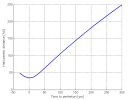
However, the simulations suggest that it would take the swarm only 13 years to begin impacting the inner solar system, so the timespan implied by the above (a few decades) would be incompatible with this scenario.

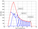
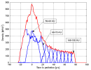
What is interesting, the energy fluctuates widely even for such small bodies. The maximum is in thousands of kilotons. But for such small bodies the probability is high that they will disrupt in the atmosphere. But of course that depends also on their composition.

Click to expand...

Indeed. That's what I was thinking: since it's the kinetic energy that does the damage, and K = 0.5mv2, energy will be highly stochastic with time due to the velocity dependence, while the impact number will be a much smoother function of time. Obviously, the majority of them will break up in the atmosphere, although this will depend on mass and impact angle as well as composition. However, even the airbursters might still do substantial damage at ground level. Hydrodynamic simulations have shown that even when the comet does not physically reach the ground, the supersonic vortex generated by the impact with the atmosphere can do so, as a supersonic blast hotter than the surface of the Sun.

_https://craterhunter.wordpress.com/the-planetary-scaring-of-the-younger-dryas-impact-event/a-thermal-airburst-impact-structure/

So impactors could be divided into three categories, based on two kinetic energy thresholds, which I will denote K0 and Kb (for 'burst'):

1) K < K0: at most, a pretty light in the sky. No ground damage.
2) K0 < K < Kb: impactor breaks up, but K is sufficient to send a shockwave to the ground. Chelyabisnk or Tunguska type events would be in the upper end of this regime.
3) K > Kb: at least part of the impactor reaches the surface, leading to an impact crater on land or a tsunami on water.

Composition is obviously a factor. Typically comets are thought to be very low-density, largely composed of water ice, small rocks, and dust, basically fluffy aggregates. Density measurements support this. Spectroscopy of the surface does not. If the EU community is right, the comets are in fact made of solid rock, and the apparent low density is due to the gravitational field being partially counteracted by electrical charge. Then again, if the EU folks are right, the Oort Cloud doesn't exist. My personal bet is that there's a lot they aren't right about.

The next issue is impact angle i, which you already calculate (albeit in 2D, I take it). This will affect the air resistance, so in practice K0 and Kb will be functions of i (as well as composition of course).

At any rate, using the categories above, the E(t) variation could be sorted as a histogram of No. of impactors in a given kinetic energy category as a function of time. This could then be calibrated using AMS data (which will be sensitive the first category), as well as studies such as the following:

_http://adsabs.harvard.edu/abs/2015MNRAS.447..769B
_http://adsabs.harvard.edu/abs/2015MNRAS.446L..31D

I finished the 3D model. I had to determine anew the positions and velocities of the planets and of the companion so that the inclination is also correct. The companion is still in the plane of eclitpic because it seem to be the most logical choice. Also the data structure now has also z component (normal to the plane of ecliptic) for the state vectors. I have a feeling that the orbit of the companion is not correct so perhaps I will modify it in near future. I forgot that the companion precesses so the current orbit is an orbit few orbital periods old. But it was only a guess anyway. For now I just leave it as it is and do some preliminary calculations.

Well of course if time permits we will get also to the impact energy as a function of time histogram. I see psychegram where you are getting at with this and then we can make some calibration. I think an output that would be of help to others should be the aim so I will try to explain everything the best I can and post some explanatory pictures.

For now I only tested the model whether it behaves correctly. And as seen in the attached pictures it seems to be ok. In the pictures the companion is seen to interact with few layers of objects that are 130 AU to 150 AU distant from the sun. And as expected now the layers are transformed into spherical formation and the structure is coherent. It is hard to visualize this on a 2D screen because everything looks so flat. So there are different views. The companion is in the centre of the sphere and everything that precedes him can be regarded as the primary wake. The density can also be interpreted. As the sphere expands the primary wake is getting less and less dense whereas the destabilized tails seem to be much denser.

Well in the next step I try to repeat the two dimensional influx experiment and see how it compares to the 2D results posted above.

tohuwabohu said:

I finished the 3D model. I had to determine anew the positions and velocities of the planets and of the companion so that the inclination is also correct. The companion is still in the plane of eclitpic because it seem to be the most logical choice. Also the data structure now has also z component (normal to the plane of ecliptic) for the state vectors. I have a feeling that the orbit of the companion is not correct so perhaps I will modify it in near future. I forgot that the companion precesses so the current orbit is an orbit few orbital periods old. But it was only a guess anyway. For now I just leave it as it is and do some preliminary calculations.

Well of course if time permits we will get also to the impact energy as a function of time histogram. I see psychegram where you are getting at with this and then we can make some calibration. I think an output that would be of help to others should be the aim so I will try to explain everything the best I can and post some explanatory pictures.

For now I only tested the model whether it behaves correctly. And as seen in the attached pictures it seems to be ok. In the pictures the companion is seen to interact with few layers of objects that are 130 AU to 150 AU distant from the sun. And as expected now the layers are transformed into spherical formation and the structure is coherent. It is hard to visualize this on a 2D screen because everything looks so flat. So there are different views. The companion is in the centre of the sphere and everything that precedes him can be regarded as the primary wake. The density can also be interpreted. As the sphere expands the primary wake is getting less and less dense whereas the destabilized tails seem to be much denser.

Well in the next step I try to repeat the two dimensional influx experiment and see how it compares to the 2D results posted above.

Click to expand...

Nice! 3D is always a pain, and the insights gained may or may not be worth all the extra effort.

Re: the discussion of impact energy, number of impactors that reach the ground, etc., I came across this on astro-ph a week or so ago:

"New methodology to determine the terminal height of a fireball"
_http://arxiv.org/pdf/1502.01898v1.pdf

I haven't given it a close read, but it seems they're able to very closely match the terminal heights of various kinds of space debris. The math doesn't look too hairy, either (famous last words?)

Re: the discussion of impact energy, number of impactors that reach the ground, etc., I came across this on astro-ph a week or so ago:

"New methodology to determine the terminal height of a fireball"
_http://arxiv.org/pdf/1502.01898v1.pdf

I haven't given it a close read, but it seems they're able to very closely match the terminal heights of various kinds of space debris. The math doesn't look too hairy, either (famous last words?)

Click to expand...

Well the article is great I studied it a bit and I think the math is just high school stuff so it's not a problem. The problem might be the unknown coefficients alpha and beta. They were derived from the observations but we should do it the other way around - calculate the trajectory and terminal height/velocity from the known coefficients. But perhaps I can sample the coefficients as a random distribution. I found also articles about 'pancake model' which could also help in predicting the impact energy. The math is very similar. This is without doubt very interesting and I will try to implement these ideas later. For now I will concentrate on the atmospheric entries so we have something that can be compared with observations and then I can extend it by taking into account the drag and heat ablation.