Computational modelling of the companion star and its interaction with Sol

So I finished the 3D simulation which was done in the same manner as the 2D one posted above. I was facing few problems with the patch shrinking in the direction normal to the plane of ecliptic which caused that the prescribed spatial density of the patch changed over time. This was solved by enlarging the patch in the normal direction so that when it meets the companion the size of the patch is decreased to the desired one and the spatial density at the moment is known. I also introduced random deviations so that the distribution is closer to the reality where the objects have different inclination and eccentricity of the orbit.

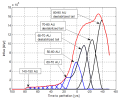
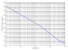
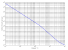
After the initial issues were resolved the tests were performed exactly as before - there were ten patches with heliocentric distances ranging from 50 AU to 150 AU with thickness of each patch being 10 AU in the radial direction. Other dimensions of the patches were chosen in such way that the formed primary wake and the destabilized tails covered the inner solar system. Thus the influx into the solar system can be accurately estimated.

The initial density of the asteroid cloud was 1e6 AU-3 (i.e. there is million bodies in a cube with dimensions 1x1x1 AU). This is the density when the patch came into the interaction with the companion. It was already shown that the influx into the inner solar system is linearly dependent on the initial density thus the results can be scaled to any other initial density or even to density that is variable with the heliocentric distance.

For this simulation also the destabilized tails were captured for distances 90 AU and less because they kicked in early enough. If also the destabilized tails for regions beyond 90 AU were captured then the influx would continue to increase. Nevertheless in this simulation the influx decays after the patches pass through the solar system. All in all a time window of 150 years was captured with 50 years for after the companion passed the perihelion. But due to the above mentioned reasons the results are valid to approximately 30 years after perihelion.

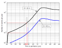
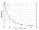
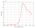
The results are shown in Fig. 17. The curves are color coded - blue is the primary wave, black are the destabilized tails and red is the overall influx obtained by superposition of all patches (the curves were simply added together). The curve is read from left to right with negative values on the x-axis corresponding to period after the companion passes perihelion.

One can clearly see that the influx is fairly constant until approx. 30 to 40 years before perihelion and is very low. Perhaps this influx can be compared to the background influx which is permanently ongoing due to the collisions and planetary interactions.
For example the influx at 30 years to perihelion is 102,400 bodies per year. The influx for 40 years to perihelion is 81,500 bodies per year.

Afterward there is steep increase in the influx and during the perihelion the influx is 1,114,200 bodies per year. This is rougly 10 times more compared to the 30-40 years to perihelion period!
The question is where on the curve are we now?

Clearly the rise in the influx is more dramatic compared to the 2D model. This is because of the contribution from the objects that were initially offset from the plane of ecliptic. For the 60-70 AU patch the primary wave and the destabilized tail are not separate events nonetheless the contribution from the destabilized tail is colored black. One can observe that the primary wave is the main contributor up until the companion reaches perihelion. Afterwards the tails kick in and the influx is almost doubled. The situation is most logical because the tails are formed behind the companion while the primary wave is always a precursor to the approaching companion. The 50-60 AU patch is not colored black but the propagation is closer to the propagation of the destabilized tails.

I was already thinking that the influx into the solar system should be directly proportional to the probability of impact and/or atmospheric entry but the relationship was unknown. Therefore I verified this theory by two independent approaches in order to determine the relationship.

The first one was simply an idea that if there is some flux in a large crossection (in this case the inner solar system) then there should be proportionally smaller flux in some smaller crossection (meaning the earth). Therefore the ratio of the crossections should be equal to the ratio of the fluxes.

The second approach was more elaborated one. Because of small initial density of the asteroid cloud there were no impacts recorded in the simulation. Therefore I increased the radius of the earth to account for atmosphere. In this way I could count the atmospheric entries which were already present in the simulation. I did this for various 'altitudes' and constructed a function relating the number of atmospheric entries which were present vs. the altitude. Then I could determine the number of impacts by extrapolating the function to zero altitude which presents the earth surface.

Both approaches gave similar results so I used the simpler one to construct the curve showing number of impacts per year (Fig. 18). In this case there is no atmosphere so the ablation is neglected thus this can be viewed as number of atmospheric entries with potential to reach the earth surface. The curve is valid for the initial density 1e6 AU-3 which should correspond to objects with several hundred meters in diameter. It is known that there is only few pluto sized objects in the Kuiper belt and with smaller sized objects the number of occurences exponentially increases. Of course it is necessary to determine the real density of the variously sized objects and then the number of atmospheric entries can be determined for wide range of object sizes.

What the curve shows is that at 30 years to perihelion the number of impacts per year is 0.0004
and at perihelion the number of impacts per year is 0.0044. Because the initial density corresponds to several hundred meters sized objects it can not be expected that they will impact the earth every year therefore taking the inverse value is more appropriate.
Taking the inverse value it can be stated that if the companion is at 30 years to perihelion there would be one impact of several hundred meters sized body per 2500 years. And at perihelion the average interval between impacts would be only 227 years. It can be concluded that the increase in the number of atmospheric entries corresponds to the increase in the influx.

At first I was thinking, those numbers seem far too low. But these are for objects with a diameter of several hundred m, which so far as I know we haven't been hit by recently, so probably it makes sense but also, direct comparison with observations is difficult using such large objects.

If we assume a power law in object size, and assume that this curve can be extrapolated in a straightforward way, what can we say about smaller objects, down to the order of 10 m, i.e. about the size of the Chelyabinsk object? Extrapolation to smaller objects (O(1 m) or so) could also make a direct comparison with the AMS and Japanese data much easier.

At first I was thinking, those numbers seem far too low. But these are for objects with a diameter of several hundred m, which so far as I know we haven't been hit by recently, so probably it makes sense but also, direct comparison with observations is difficult using such large objects.

If we assume a power law in object size, and assume that this curve can be extrapolated in a straightforward way, what can we say about smaller objects, down to the order of 10 m, i.e. about the size of the Chelyabinsk object? Extrapolation to smaller objects (O(1 m) or so) could also make a direct comparison with the AMS and Japanese data much easier.

Click to expand...

That is exactly what I was thinking. I have been going through a lot of papers so that I could make some estimate on the density. Mostly only some limits are given for numbers of very large objects based on the assumed total mass of the oort cloud or kuiper belt. But because I do not know the volume of these formations it is of no use. Besides the spatial density will surely vary with distance. There might even be areas with high density and low density.

Nevertheless after reading many papers I found one which looks promising. It is based on occultation study and I think that good approximation is made in the paper. The problem is that compared to some other papers there is large uncertainty up to one order of magnitude. Thus I am not sure about the accuracy but I will put the numbers together and post the results tomorrow.

So I was able to reconstruct the spatial density distribution of the kuiper belt objects according to [1]. In the paper the size distribution is presented which agrees with observations and also simulation results for objects varying in diameter from 10 m up to over 100 km.

I adjusted the size to represent diameter of the body rather than radius and recalculated their numbers to spatial density, i.e. number of objects per cubic AU. This is cumulative distribution so the number referes to number of bodies with given diameter or larger.

For example in previous posts I made simulations with spatial density 1e6 AU-3. Looking at the graph in Fig. 19 one can see that to the density 106 corresponds diameter 0.4 km. That is there is one million bodies in a unit AU cube with size 400 m or larger. I don't know whether this is accurate but it seems to be reasonable. Fig. 19a shows only a portion up to 1 km diameter with finer detail and with diameter in meters. So for small objects up to 0.1 m one can determine their spatial density.

I checked the curve also with other papers and it seems to be in good agreement. But there are some deviations so we will see what it will look like after I recalculate the relationship for number of atmospheric entries.


References:

[1] Schlichting, H. E. Initial Planetesimal Sizes and the Size Distribution of Small Kuiper Belt Objects. J. Astron. 146, 2013.

The number of atmospheric entries was calculated for reference point 30 years before perihelion. It's a point on the end of the relatively constant region according to the curve in Fig. 17 and Fig. 18. Therefore the number of events should gradually increase after this point so we should start quite low.

But the results in Fig. 20 tell different story. It is a common knowledge that Chelyabinsk event sized body (just under 20 m diameter) on average impacts earth once every 10 years and Tunguska event sized body (approx. 50 m) impacts earth once every 100 years on average.

Looking at Fig. 20 one can observe that 20 m sized body should enter the atmosphere 2 times per year and 50 m sized body once every 10 years. It seems that this is not what the observations are saying. The results are off by one order of magnitude.

Well I have been thinking about it and pondering where I did go wrong since yesterday. Clearly the number of atmospheric entries depends on the spatial density of the asteroid cloud and on the heliocentric distance of the companion star. And what I think is that the size distribution and spatial density is more or less correct and I think also that the simulation gives good results but of course the results depend on the input.

One should keep in mind that the simulation assumed constant spatial density of the asteroids which of course is idealized case. In reality the density varies with heliocentric distance. There can even be regions with very small density followed by regions with above average spatial density.

Therefore the simulation overestimates the observed frequency of atmospheric entries because the asteroid cloud was modeled as continuous region with constant density. In reality the density should exponentially decrease with distance. So this is what is neglected in the simulation. Nonetheless the results are still valid and give some kind of upper limit of possible number of events. If the companion star would hit region with density corresponding to that measured at 40 AU from the occultation study and also used in the simulation, then the number of impacting bodies would be in agreement with the simulation results. At least that is the conclusion that can be made based on logic.

So another step would be to expand the simulation to take into account also the spatial density distribution along the heliocentric distance. For now only the distance of the companion has been taken into account thus it is not possible to make any comparison with the observed influx.

You're making remarkable progress, tohuwabohu.

After reading your latest post, my question would be whether you suppose that all incoming bodies would hit earth atmosphere or that most of them would end up passing along with no harm done, and only a few (relatively speaking) of a swarm --coming in like waves or distinct salvo's-- would actually hit earth ?

That could account for the discrepancies found, I think; unless I'm missing something.

Palinurus said:

You're making remarkable progress, tohuwabohu.

After reading your latest post, my question would be whether you suppose that all incoming bodies would hit earth atmosphere or that most of them would end up passing along with no harm done, and only a few (relatively speaking) of a swarm --coming in like waves or distinct salvo's-- would actually hit earth ?

That could account for the discrepancies found, I think; unless I'm missing something.

Click to expand...

Thank you Palinurus, I will try to explain as best as possible. Well looking at Fig. 15 and Fig. 16 one can see that if the asteroid cloud is quite large then after the interaction with the companion it transforms into spherical shape. Because I wanted to reduce the calculation time I model only part of the asteroid cloud (a patch) that interacts with the inner solar system, that is after the interaction with the companion the patch expands into such dimensions that it covers (is larger than) the inner solar system when it passes through. Therefore only very small fraction of the bodies enter the atmosphere and potentially impact the earth. So you are correct with the salvo effect.

Looking at Fig. 17 one can observe the influx of the bodies into the inner solar system per year for initial spatial density of the asteroid cloud 1e6 bodies per cubic AU. The influx is in hundred thousands bodies per year.
Comparing the influx to the number of atmospheric entries per year for the same initial spatial density (Fig. 18), one can observe that only one in 250 million bodies (roughly) will impact the earth. So the fraction is very very small but I think it is reasonable.

Well in the meantime I did also simulations with density that is decaying with increasing distance. And I think this will help. I will post the results shortly but first I have to crunch through the data and create some useful pictures.

If you have some other questions or suggestions feel free to chime in. I will be glad to help.

Thanks for your explanations, tohuwabohu. I feel like having better grasp now on what you're doing. No further questions or remarks ATM. Carry on! ;)

In order to introduce spatial density decaying with heliocentric distance, new variables had to be defined. Firstly I took the density at 40 AU from dr. Schlichting as base density. Secondly, based on the models of Oort cloud formation (DQT87, DLDW - references [1], [2] in reply #66) I assume that the density decays exponentially with logarithmic exponent -2.5 (Fig. 21). There is uncertainty in the value of the exponent because for Kuiper belt region the density distribution might be different. But I take the value as an average.

The influx was constructed as linear combination of small slices with different densities according to the abovementioned density distribution, which serves as a weighing function. I divided the whole radial thickness of 100 AU into 1 AU slices. Thus there are 100 onion-like layers. This is advantageous because any linear combination can be used to reconstruct the influx and therefore also number of atmospheric entries. It is even possible to use arbitrary spatial density distribution but this is pointless because the exact density profile is not known therefore it would be only a guess. On the other hand the presented logarithmic distribution can be taken as an average spatial density distribution.

Other parameters of the simulation were unchanged so the results can be directly compared to the simulation with constant density. The influx curve is presented in Fig. 22. There are two things that are evident on first sight. The first is that the slope before perihelion is much steeper because the influx rises with double exponential. It was shown that the influx increases substantially even for asteroid cloud with constant density due to the companion proximity nonetheless now also the density increases in addition to the diminishing distance.

The second observation is that the maximum is now just after the perihelion. Afterwards the influx decreases. This is because the tails that arrive after the companion have also reduced density. Remember that the tails arrive in reverse order compared to the primary wave. The tails closest to the sun arrive first and are followed by tails corresponding to patches with larger and larger heliocentric distance and because the spatial density decays with increasing heliocentric distance, also the influx decreases.

Anyway there will be mayhem even before the companion reaches perihelion. If we take the point at 20 years to perihelion for reference then at perihelion the influx is almost tenfold. This means that there is also ten times larger probability of impact. An event that would happen once in ten years would happen once a year. This is significant change in just 20 years. I think we can now proceed and estimate (although only roughly) the distance of the companion.

Brilliant. The pieces have come together quite beautifully. This could actually make quite a nice paper, when it's complete! (Assuming it could get past peer review, that is ... odds are perihelion will have come and gone by the time that happens ;) ) Still, this work practically demands greater visibility than it's likely to get on the forum. I'd strongly suggest writing it up as a SOTT Focus article, with maybe an ArXiV paper for the more technical details.

The sharp slope near perihelion is quite terrifying. Basically indicates that we get practically no warning until it's on top of us, and then blammo, TEOTWAWKI.

psychegram said:

Brilliant. The pieces have come together quite beautifully. This could actually make quite a nice paper, when it's complete! (Assuming it could get past peer review, that is ... odds are perihelion will have come and gone by the time that happens ;) ) Still, this work practically demands greater visibility than it's likely to get on the forum. I'd strongly suggest writing it up as a SOTT Focus article, with maybe an ArXiV paper for the more technical details.

Click to expand...

Yes, I agree wholeheartedly with you psychegram. This work deserves a wider audience and a thorough presentation.

psychegram said:

The sharp slope near perihelion is quite terrifying. Basically indicates that we get practically no warning until it's on top of us, and then blammo, TEOTWAWKI.

Click to expand...

Agreed. I've reread the whole thread the other day to increase my focus. The period of perihelion would take about sixty years in order to complete the full curved trajectory around the vicinity of Pluto's orbit, as was stated in the beginning. We are confronted with a notable increase in 'hits' already now, but a tenfold increase of the current level --or even more for that matter-- seems hardly imaginable. That could drive unsuspecting people completely crazy, I think. The end of the world as we know it. Indeed !!

The thing is I started to write what is in this thread as a paper. And the paper is now 26 pages long.
And there is still a lot of stuff to do. But I don't think any journal would be interested because this topic is sensitive. And I agree with you guys that these things deserve wider audience and that is why I started this thread. The other thing is I am not all knowing and any input is much appreciated so together we can accomplish something. Or at least make few steps forward which will help someone else to get to the finish so to say.

As you see it was a long journey to come to this point and basically, yes it's kinda mosaic with plenty of pieces that had to be gathered and put togehter. And there is so many variables and it seems everything is interconnected so that sometimes it's really hard to keep all these things in my head. Nevertheless I think that now indeed the pieces start to fit together. I already did some preliminary calculations and the companion distance can be estimated. But there is always a possibility that I missed something or made some unfortunate assumptions so without an independent confirmation I am hesitant to write an article for SOTT because we all know that SOTT is great because it values facts and news based on facts.

But don't get me wrong, I think that we have made some great progress and I think this thread goes in the right direction. And even if we do some small mistake it's not a problem because we can always correct our course. So perhaps we are not there yet but surely we are getting closer to our goal. And when the time comes I will be glad to write an article.

Utilizing the knowledge from the simulations and also using the size distribution and spatial density distribution it is possible to construct impact curve for arbitrary sized object. I think that returning to the post where I mentioned some general observations from the Chelyabinsk and Tunguska events can be useful. I decided that because the recurrence of these events is roughly known I can construct the impact curves for both these events and then compare it with the observations.

So I took the influx curve, size distribution and density distribution and created two impact curves. One is for 20 m sized objects and the other one is for 50 m sized objects. They are both in Fig. 23. I had to make the y-axis logarithmic because it was not readable otherwise. The change in impacts with time is quite large and spans over two orders of magnitude for each curve.

Now we can estimate where we are by locating the number of events per year on the y axis for each curve. We can move along the curves so going closer to perihelion means also more events per year and going the other way along the curve means decrease in the number of events. Thus we can pinpoint the time to perihelion that corresponds to the number of events. I did this for both curves in the figure and surprisingly both of the results are in good agreement and converge to value 32.9 years to perihelion.

Thus we can pinpoint the time to perihelion that corresponds to the number of events. I did this for both curves in the figure and surprisingly both of the results are in good agreement and converge to value 32.9 years to perihelion.

Click to expand...

This estimate should be taken as an upper limit because clearly if there is a gap in the asteroid cloud up to say 10 years before perihelion then we would not notice significant increase in the influx. Only after the companion reaches dense region we would notice dramatic increase and it would hit us with full power without a warning. So clearly I can not exclude the possibility that the companion is closer to perihelion than the estimate.

There is also possibility that the companion is further and the estimate is pessimistic. But this would be limited by the uncertainty in the density distribution function and size distribution function. These uncertainties are not known but they are finite. On the other hand if the companion is closer than the estimate, no lower limit can be placed on its heliocentric distance. We can limit it only by assumption that if it would be at perihelion it would be visible and/or detected.

According to the simulation the heliocentric distance of the companion corresponding to the 32.9 years to perihelion is 50 to 55 AU depending on the exact perihelion distance.