Computational modelling of the companion star and its interaction with Sol

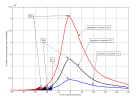
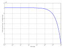
Now that the true flux is known we can have a look at how it compares with the impact curve. Note that the impact curve depends on the density distribution function and on the minimal size of the observed objects. So these parameters can be modified when trying to make a fit.

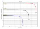
After few hours of trying it became obvious I could not do it. If you look at the histogram in Fig. 31 – the one constructed from the AMS data, you can notice that there are two distinct slopes in it. The first is spanning the years 2005 to 2010 and the second is from 2010 to 2013. Well there is also third slope for years 2013 and 2014 but I found that this slope corresponds to constant density profile.

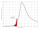
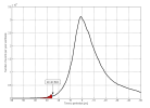
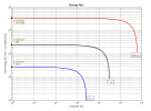
As you can see I could make a perfect fit with the first one and the impact curve albeit I had to push it a little bit to the right (closer to perihelion) and increase the logarithmic exponent to -4.9 (Fig. 32). This is the lower bound that was clearly defined because for smaller exponents (in absolute terms, meaning closer to zero) the error of the fit started to rise dramatically.

For this fit our position is 15 years before perihelion so in other words if it were true then the companion would reach perihelion in year 2030. The number of fireballs at maximum near perihelion would be 5 times higher compared to what it is today.

I could also identify in the same way the upper bound for logarithmic exponent -6.6 and the result of the fit is shown in Fig. 33. One can clearly see that the AMS histogram is shifted to the left and there is also larger flux at the perihelion because of this.

The possible position for us if the fit would be correct is marked by the point with the sign 'we are here' but there should be a big question mark because there is no way to know. For the upper bound the companion needs 25 years to reach the perihelion.

MusicMan said:

Hello tohuwabohu, that Figure 31 is pretty scary, as it looks like it is becoming hyperbolic.
One could only hope that it represents the top of a bell curve.
I couldn't believe the number of variables you had to consider when working it out.
Great work.

Click to expand...

Hello MusicMan, I think that you might be right. If you look at Figure 32 then the black curve represents an average number of events therefore it might be possible that in the coming years the number of events will perhaps decrease or stagnate to reach the black curve.

In theory if the black curve is right then the AMS data should oscillate around the curve. So we might wanna wait few years how the situation develops. For now the year 2015 from AMS looks similar to 2014.

To verify whether the bounds are correct I also approximated the somewhat bumpy impact curve from the simulation by smooth function so as to eliminate possible errors arising from the unevenly changing slope of the curve. And I found that there is global minimum in the error for logarithmic exponent -6.2.

This is the best possible fit that was found across the whole range of logarithmic exponents for the density function and of the time to perihelion value by minimizing the error of the fit. The impact curve for bodies with size above quarter inch was just perfect for this.

I have to note though that the error function has flat bottom thus it is possible to shift the position of the AMS data by 5 years up or down with only slight increase in the error. But this is already covered by the lower and upper bounds which are in good agreement with the mean value obtained for a smoothed curve. I have put the mean value with the bounds into one image for comparison (Fig. 34).

So the mean value is 20 years left before the companion reaches perihelion. I do not know whether this is large or small value but the fit was clear. The uncertainty here is the average slope of the AMS data. It would be necessary to wait for another 5 to 10 years to improve the value of the average.

One can clearly observe the increase in the number of fireballs at the perihelion compared to what is now with the shift of the 'we are here' position to the left, i.e. farther from the perihelion. Whereas if we are 15 years distant from the perihelion the number of events will increase only 5 times, for 25 years distance to perihelion there will be 34 times more fireballs.
Keeping in mind that this is one in 26 million years event I am somewhat inclined toward the larger values.

Also of interest is the fact that because the impact curve had to be scaled by the same amount as the AMS data, it does not matter whether the total fireball flux estimate from the probability of observation is accurate or not. The only thing that could be fit was the slope.

So as I said the first slope spanning the years 2005 to 2010 could be fit by increasing the logarithmic exponent. But I could not fit the second slope no matter what, because it is so steep that such slope can't be found anywhere along the curve!

As of now I can think only of one reason why the fit is not possible:
The companion hit an asteroid cloud with above average density that resulted in way steeper slope than the average impact curve can handle.

To resolve this problem I could only adjust the density function to match the observations. But this would not help us to predict anything because this can be done only after the event already happened.

Second solution is that I can adjust the exponent and perhaps also the base density, but because I do not know to what value it would be only a guess. The thing is, I don't know whether the first slope is the average and the second slope is the anomaly in the AMS histogram or vice versa. If the first slope is the average then the results are very good. But if the first slope corresponds to a gap then the average might be somewhere in between.

We are interested in average because we do not know the exact density profile of the asteroid cloud. But taking the average we can say that the real flux will oscillate in some limits around the average thus some predictions are possible.

So I guess that without an external help I can not move further. The only thing I can do is to wait few years to see how the situation develops.

Well the situation in the world is dire and I cannot imagine it will last. So perhaps there is possibility that the companion is closer than the estimate. And I am aware there are also other possibilities that are tied to multi-density and multi-dimensional universe.

So as I said the first slope spanning the years 2005 to 2010 could be fit by increasing the logarithmic exponent. But I could not fit the second slope no matter what, because it is so steep that such slope can't be found anywhere along the curve!

As of now I can think only of one reason why the fit is not possible:
The companion hit an asteroid cloud with above average density that resulted in way steeper slope than the average impact curve can handle.

Click to expand...

There is another possible explanation I think, which is somewhat similar in some respects: according to the C's the arrival of the companion star is supposed to coincide this time with the advent of the comet cluster which allegedly has a recurrence rate of about 3600 years. Therefore it's conceivable that the companion star somehow accelerated several of the bolides from that cluster into an early arrival trajectory.

Just a thought. FWIW.

Tohuwabohu:

I'm glad the probability analysis worked out, and very impressed by the work you've done implementing it. Those numbers are stunning, though ... that's really just a huge influx of cosmic material. I wonder what contribution it might be making to the atmospheric heat budget? It could be interesting to see how much energy (assuming a mean kinetic energy per event) and material (assuming a mean mass, and total disintegration). Comparisons could then be made to volcanic input. Could go quite a way towards explaining the 'anomalies' in climate we've been experiencing.

Palinurus:

That's a very good point you have, regarding the 3600 year period cometary debris cluster. Quantifying its contribution might prove difficult, though. My understanding is that there are two origins for this phenomenon which have been suggested:

1) resonance induced by Nemesis (I believe this was the C's suggestion)
2) the remnants of a giant comet (Clube & Napier's hypothesis, if I recall correctly).

Hypothesis 1) could perhaps be constrained numerically, by running N-body simulations over multiple cycles of Nemesis' orbit. I say 'perhaps' because I expect it would be impractical, given the run-time of such a simulation. Although, perhaps a much coarser simulation could provide the needed insight.

Constraints on hypothesis 2) might have already been provided by Clube & Napier. Not having read their work myself, I don't know how detailed their historical reconstruction of the giant comet's mass, orbit, etc., was. However, I expect there may be some on the Forum who have more specific knowledge than I.

I think I might be able to calculate the yearly mass deposit on earth from the incoming bodies and also the energy that is related to it. But I am not sure about the periodic cometary swarm. Such calculation would take few months to finish and the resolution would have to be very low. We are talking perhaps about one thousand bodies. So the results might be inconclusive.

So first I try to calculate the yearly statistics and then I will have a look at the 3600 year period.
I am thinking that for the statistics I can utilize the distribution in Fig. 24. I have to extrapolate it though to include also very fine dust particles. And then it is only a matter of integration.

I do not know psychegram what you intend to do exactly with the volcanic activity. Can you write in some more detail about it?

Mass flux

As psychegram said it might be interesting to calculate the total mass that is deposited into the atmosphere due to the incoming space rocks. I assume that all incoming bodies are chondrites with 10 percent porosity for simplicity thus I will use density of 3400 kg/m3 to convert the mass of any object to its size or vice versa.

The first thing I am curious about is whether the most mass comes from the small dust like particles or from large objects. The large objects will disintegrate either completely or partially so in the end the atmosphere will be loaded by dust no matter what. And it will then take some time for the dust to settle. I will come back to this later, for now I have taken the extended curve and divided it into small bins according to mass of the rocks. Each bin is spanning one order of magnitude. The overall mass ranges from micrometer sized particles to several hundred kilometer sized bodies. Then I basically integrated numerically the cumulative curve for each bin according to the y-axis because we are interested in total mass in the bin.

The result in shown in Fig. 35. It is clear from the figure that the smaller particles even though they are more abundant contribute with smaller mass overall. And with increasing mass of the space rocks also the total mass deposited per year in each bin increases. So the large rocks burden the atmosphere more than the smaller ones.

And because of this an interesting question arises. It is related to what was mentioned before with the settling of the dust. The question is where should be the cutoff for the mass of the rocks. Because I am taking yearly deposit there are only bodies of certain size that are truly impacting earth at least once per year. The larger bodies will impact earth once per tens or even thousands of years. So I can take an average in the case of large bodies where I simply spread the total mass over the period it takes for such bodies to strike again.

So for example the Chelyabinsk sized body should impact earth once per 10 years. So I can take its overall mass and distribute it over the 10 years. It will be averaged whereas in reality there will be large spike in the atmospheric dust and it will then settle down gradually over time.

So what I did next was I took the one order of magnitude divisions in the cumulative distribution and divided them into smaller segments up to ten per division. Then each thus obtained segment was divided into very small chunks for numerical integration and the result was saved in each segment. To obtain the cumulative distribution the value in each segment was accumulated from the largest mass to the lowest.

And the result is shown in Fig. 36. This is actually complementary cumulative distribution over the whole mass range. What this curve means is that the y-value corresponds to the total mass flux for bodies of size equal or larger than is given by the value on the x-axis. So the value on the left end of the curve is the total mass flux over the whole mass range of the incoming rocks. I verified the result by analytical integration and both methods converge to the same value. So I take it is accurate based on the input.

So to conclude, the total mass flux into the earth atmosphere is approximately 714 million kg per year.
This boils down to 714 000 tons of material per year. This is quite low value I was expecting much larger influx. But of course the value should also increase from year to year with the flux of the bolides.

As I am thinking about it the value is definitely correct what is not clear is in what year is it correct. :)

While I am at it I also constructed curves that are valid when only smaller rocks are taken into account. I added it to the existing one and changed the x-axis to read the size of the rocks (Fig. 37).

So for example if we take only rocks that impact earth at least once a year then the total deposit is only 5656 metric tons. For rocks up to one kilometer in size the total deposit is 50860 tons. These values are of course averaged over the period of impacts. For example 20 m sized body has mass over 14,000 tons. But because it impacts earth only once per ten years it contributes to the average yearly flux only by 1,400 tons.

For some reason I think that these values are most conservative and in reality the flux is larger. But these values are tied to the observations of the number of events per year. So if the periodicity of the impacts is correct then there might be also another thing to consider and that is the loading of the inner solar system by dust from the cometary passages. The dust would be in turn deposited into the atmosphere especially into the upper layers from which it would precipitate downwards.

tohuwabohu,

Although I am not of the scientific bent, I appreciate all the hard work you are doing. The estimate of 20 years before a dramatic increase of possible impacts is sobering. I do get the drift of some of the charts even though I don't begin to understand the enormous work it takes to produce them. I am also appreciative of the other posts and comments and I am really impressed with the quality of brain-work being done. It's kind of like a "brain pool" instead of a "brain drain"!

I will keep checking back to see how things progress.

Thank you,

goyacobol :)

Thank you so much goyacobol for your words of support. I was just wondering this morning whether this thread is of help to anyone and bang here comes you with your cheerfull words. This means very much to me especially if you are not from scientific community.

I am trying to explain everything as simply as I can but of course it is hard because it means to put the knowledge on the paper. And many times what is common knowledge for me might be not so common for others. For me to do something is the easy part even if it requires lot of effort and lot of studying. But to explain how I did it that is the real challenge for me. I am aware of this and therefore you or anyone else is welcome here to ask questions and write some suggestions and I will be happy to explain or follow some leads.

Just recently I was hesitating what direction should I take next after the time to perihelion estimation. And without the suggestions from Palinurus and psychegram I would be scratching my head even now.

So any input is very much appreciated and I will continue to contribute to this thread. We have already established the mass flux and I am working already on the energy flux. So I will post the results later.

Energy flux

If we assume that the kinetic energy of the fireballs will dissipate in the atmosphere upon the entry then we can calculate total energy per year due to the incoming bodies. I used similar process that was also used to determine the mass flux. Only the black energetic curve in Fig. 25 was taken and was integrated along y-axis. Thus the average impact velocity is taken to be 20.3 km/s.

The results are presented in Fig. 38 in the same fashion as for the mass flux only now the total energy is shown on the y-axis. The total energy for the whole range of bodies up to 400 km in size is 35 Mt per year.

This is a respectable value because for example tunguska event which was caused by a 50 m sized meteor released energy approximately 10 Mt.

If we take only the bodies that will impact earth at least once per year then their combined energy is only 278.5 kt. This is only half of the Chelyabinsk event.

I think volcanoes can release energy in Mt but more than that they do eject ash in millions of tons. Something similar would happen if a meteor would strike earth, it would eject massive amount of ash and dust. But for now we have no evidence nonetheless it can be calculated. So it seems that we are squeezed from above and also from below.

So I will leave the comparison with the volcanic activity on you psychegram if you are interested. And I will move onto the periodic cometary swarm.

Here is nice compilation of the transcripts referring to the companion star and the comet cluster, thank you thorbiorn.

http://cassiopaea.org/forum/index.php/topic,8401.0.html