Computational modelling of the companion star and its interaction with Sol

[tohuwabohu]

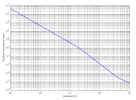
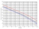
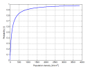
I also created the curve showing number of events in relation to the object size for the estimated time to perihelion 32.9 years. I will take the estimate as the reference point and perhaps we can try to find some database with number of impacts for different object sizes. In this way we could see whether there is good agreement with observations along the curve. If not then we can estimate some kind of interval in which the ETA of the companion might be. I might wanna look at the AMS database first.

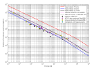
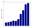
I will also try to construct the energy histogram curve that is similar to that in Fig. 24 but with energy in kilotons on the x-axis instead of asteroid size. The problem is that the velocity of the incoming objects is independent of their size thus it can be anywhere from 13 km/s to 73 km/s upon atmospheric entry. In scientific papers there is a convention to take average velocity 20.3 km/s but this would underestimate possible energy of the incoming objects.

 

[tohuwabohu]

So let us construct also the energetic histogram, that is, the number of events given by the kinetic energy of the bodies upon entering the atmosphere. This is hard to construct exactly because the kinetic energy depends on the mass of the body and also on its velocity. The mass is proportional to the size of the object and its density so there is no problem. But the velocity is independent of the object size and can vary in the range 13 km/s to 73 km/s. Therefore for example 20 m sized body with high velocity can have equal kinetic energy to 40 m sized body with low velocity. The problem is that even though low energy impacts should be more frequent, the number of atmospheric entries per year is tied to the size of the objects as shown in Fig. 24. Thus a paradox is present because even though the probability of impact is given by the influx of the bodies of given size, the energy is also given by velocity which is unrelated to the size and therefore the energy can be higher for smaller bodies.

This ambiguity can be neatly solved by taking an average value of the impact velocities. Nonetheless it can also be solved more exactly by sampling the velocity distribution according to statistics from the simulation. But one should take care because the diffusion due to collisional scattering is neglected. Therefore the distribution is more pronounced on the tails. It resembles inverted gaussian curve. More probable impact velocities overall are the velocities with extreme values.

There is also another observation – the impact velocity also depends on the season. More precisely, on the relative position of the Earth on the orbit and that of the companion. Because the companion arrives from the direction given by 18h RA in the simulation, the extreme velocities are present during winter months and then the velocities gradually approach the mean value during summer. This is very important observation.

After thorough contemplation I decided to construct three curves (Fig. 25). The red curve was constructed by sampling the velocity distribution according to the simulation results. The procedure used is very complicated but basically what I've done is this: The cumulative size distribution was divided into buckets with similar sized objects. Then a sampling set was created in each bucket with the desired velocity distribution. Then the energy for each body in the sampling set was calculated and it was then scaled to real density and redistributed into an energy histogram.

As was mentioned above, due to neglecting some effects in the simulation, the velocity distribution is in favor of extreme values. The red curve therefore approaches the upper limit for velocity - that is 73 km/s. Therefore it should be regarded as an upper limit. This can be different for retrograde orbit of the companion. The velocity distribution is permanently shifting with heliocentric distance of the companion. With small distance the velocity distribution curve is symmetric. But with large distance the distribution is shifted in favor of higher velocity. Therefore for retrograde orbit of the companion the shift can be towards smaller velocities.

The black curve was created with scientific papers in mind where an average velocity is used. The average velocity used to construct the curve was 20.3 km/s.

The blue curve is the lower limit and the minimum velocity 13 km/s was used to construct the curve.

The plot shows number of events per year for given energy or higher. The energy is kinetic energy of the body when entering atmosphere. For now the atmospheric effects are neglected but they can be included if necessary.

 

[tohuwabohu]

I was looking for some data which could be used to increase accuracy of the model and came upon several scientific papers which handle small subsets of impact events. Some authors analyzed old AFTAC data literally 50 years old and there are others that used large events that are publicly well known but there is only handful of them. The used datasets are very limited but I would say we have no better information available. The satellite data is not publicly available in raw format. But there are papers using these data or infrasonic data but it seems that the results are quite biased toward lower values of recurrence. Most authors simply average the data over some time period and disregard the possibility that the influx changes over time. Therefore the averaged results underestimate the current influx. I even think that they want to convince us that the influx is constant over time.

I used the graph from previous post and inserted the data I found in the papers thus I created some kind of collage where one can compare the results from different studies (Fig. 26). Clearly most of the data is at the lower limit of the impact velocity. The infrasound bolide flux is in good agreement for larger events (>100 kt). The satellite data are averaged over 20 year period from 1994 to 2013 and thus are below the minimal impact velocity. AFTAC data are a drag. Best fit with the results presented here achieved ReVelle's analysis of 1995-2001 bolide flux. The slope is accurate and also the values correspond with the mean impact velocity and also with the Chelyabinsk and Tunguska events.

Nevertheless I think that this proves that the size distribution function used in the simulation is correct. Because overall the slope seems to be in good agreement with the other data we can consider this part of the simulation confirmed. On the other hand the density function is still not confirmed because data that are continuous in time are not available except for the AMS database. Basically this function affects the slope of the impact curve in Fig. 22 and therefore also the companion position and the ability to correctly predict the flux.

I think now is the time to check the AMS database and we'll see whether it will help us to move forward.

 

[psychegram]

So, basically, the initial wave is indistinguishable from the background level. Not so surprising, then. The agreement with the data is great.

Unfortunately, the AMS doesn't seem to offer their database in an easily machine-readable format. Going through their sitings logs by hand seems like it would be incredibly tedious. So, I've emailed them to see if they might have the data in ascii format, or .fits, or something else that can be easily worked with.

 

[tohuwabohu]

Unfortunately, the AMS doesn't seem to offer their database in an easily machine-readable format. Going through their sitings logs by hand seems like it would be incredibly tedious. So, I've emailed them to see if they might have the data in ascii format, or .fits, or something else that can be easily worked with.

That would help tremendously. There is a lot of events starting with 2005. The yearly count of the fireball events can be obtained easily so I will start with that while we are waiting. And when the data in suitable format will be available then we can do some detailed analysis.

 

[psychegram]

Unfortunately, the AMS doesn't seem to offer their database in an easily machine-readable format. Going through their sitings logs by hand seems like it would be incredibly tedious. So, I've emailed them to see if they might have the data in ascii format, or .fits, or something else that can be easily worked with.

That would help tremendously. There is a lot of events starting with 2005. The yearly count of the fireball events can be obtained easily so I will start with that while we are waiting. And when the data in suitable format will be available then we can do some detailed analysis.

Still haven't heard back from him, unfortunately.

In the meantime I've been thinking over how to extract maximum value from the database.

The only classifications they provide are whether there was a sighting, how many people saw it, whether there was sound, and whether there was fragmentation. I'm thinking maybe these could be used as three ascending K.E. bins, since presumably objects that break up have the most energy, followed by objects that get close enough to the ground to generate an audible sonic boom, followed by objects that burn up high in the atmosphere.

The data are also geotagged. A more sophisticated level of analysis could cross-correlate sightings with population density, as presumably the probability of an object being seen goes up with the number of eyes available in that locality to see it. This could then be used as a weighting function. Another possibility would be to separate locales by population density, or perhaps simply have a lower cutoff, and then use the surface area of that region (of course, much smaller than the entire continental US) to normalize the simulation predictions.

 

[tohuwabohu]

I found they already did some kind of analysis here

_http://www.amsmeteors.org/fireballs/fireball-tracking-system-analysis/

but it is not exactly what we need. Nonetheless there is also excel file with the data available but it is only up to 2013.

I think the kinetic energy bins are a good idea. We already have the graph with number of events per year thus it could be compared. But as you mentioned the problem is that there is good coverage only for US. What we need is the flux for the entire world. I was thinking that the simplest would be to scale the events according to landmass.

There is also another thing. Not all events are related to the companion. There are NEOs and periodic events and background flux and so on. So it would be useful to know what percentage of the events are caused by companion. So some statistics would come in handy. But perhaps because of the dramatic increase of the flux in the last few years it might be safe to assume that the flux caused by the companion is dominant.

 

[tohuwabohu]

Anyway here in Fig. 27 are the yearly data - the number of fireball events according to the AMS for last ten years. It is possible to distinguish three different slopes. Between 2005 and 2010 the slope is moderate with small hiccup in 2009. A very steep increase follows between 2010 and 2013. And it seems in 2014 only slight increase is present compared to 2013. We will see what 2015 brings but the january and february data are on par with 2014 so far.

These are only sightings that were made in US therefore overall the number of fireball events should be much larger. I will try to scale the data and will see then whether it corresponds to the impact curve.

 

[psychegram]

Oh, there is an excel file! Brilliant. Too bad they haven't updated it in a couple years, though.

I think, before extrapolating to the rest of the planet, it still might be a good idea to perform a population-density weighting. Population in the US is highly nonuniform: the east coast is very dense, the west coast mildly dense, the inland practically uninhabited in some places. Maybe in the end, comparison of sighting vs. population heat maps will show that the effect is negligible, but it would be good to know this for certain. The overall effect would be to increase the event flux.

Turning up the temporal resolution might help remove the background signal. Meteor showers tend to come at certain specific times of the year, so there should be spikes at these times. Maybe the easiest way to remove the signal would be to simply mask out these dates. It could also be interesting to see if there is any sort of regular fluctuation in the remaining data over the course of a year, i.e. if certain times of year tend to shower a higher object flux than others.

 

[tohuwabohu]

You were right psychegram the probability map was a good idea. I had to manually extract the data though which was quite tedious and therefore I used only the 2014 data for the analysis. The other years will be scaled accordingly.

Of course the idea behind it is correct - each event has finite probability that it will be observed and reported. Thus the first step is to account for the probability and to create a probability map for each of the fifty states. The landmass and population of each state were extracted from government site.

To assess the probability of observation of any event a probability function has to be constructed. The function is selected according to two constraints. First, if there is no population there is zero probability of observation. Second, the 100 percent observation limit is reached asymptotically as the population density tends to infinity.

Suitable function was found in the form y = x/(x+b), where x is the population density and b is an unknown constant that has to be determined.

The unknown constant was found through optimization procedure where the objective function to be minimized was in the form of relative error of event density from the average. The final probability function that was used for further analysis is shown in Fig. 28.

 

[tohuwabohu]

Next the population per square kilometer was calculated and the probability of observation was determined using the probability function. I constructed a probability map for better visualization in Fig. 29. And truly the probability to spot a fireball is proportional to the population per square kilometer. But this is not so surprising.

 

[tohuwabohu]

If the observed events represent only a fraction of the true count then the true flux has to be higher. Therefore the number of events observed in each of the states was multiplied by the inverse of the probability. The final number of events was obtained by summing the results for all states.

The true number of fireball events accounting for the probability of spotting the event happens to be 27562 for the year 2014. The number of observed fireballs was 3381 for the same year. Therefore overall it can be stated that the probability to spot a fireball is 12.3 % and the true number of fireballs is approximately 8 times higher than the observed number of fireballs.

 

[tohuwabohu]

Here in Fig. 30 the data are shown that were used to obtain the results.

 

[tohuwabohu]

Now also the other years can be scaled accordingly. But that is not all. In order to compare the observations with the simulation it is necessary to obtain the flux for the whole world. Summing the landmass of all of the states one comes to the value of the USA landmass which is 9,826,455 km2. Assuming that the fireballs do not prefer some country over some another, i.e. their distribution is uniform, it is possible to scale the number of fireballs in the world simply by comparing the surface area of the world with the USA landmass. The surface area of the Earth being 510 million km2, the total Earth fireball flux should be 51.9 times higher compared to the US flux.

For the year 2014 that will make 1.43 million fireballs worldwide (Fig. 31). The number is quite astounding and converting to daily value this means approximately 3900 fireballs each day.

The number seems to be very high but we should keep in mind that only small fraction of them is observed.

 

[MusicMan]

Hello tohuwabohu, that Figure 31 is pretty scary, as it looks like it is becoming hyperbolic.
One could only hope that it represents the top of a bell curve.
I couldn't believe the number of variables you had to consider when working it out.
Great work.